How to select a random result in Google Sheets

Previously, Quantrimang.com guided you to create the above random number sequence on Google Sheets. And in this article you will know more ways to choose a random result, for the purpose of drawing a winning number, or choosing a single lucky person, for example. To be able to choose a random result in Google Sheets, we need to combine many different functions in Sheets, according to the article below.

Instructions for choosing a random Google Sheets result

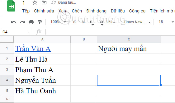
We will have a list table as shown. You will choose 1 person at random. You can choose a random number corresponding to the name or display a random name.

How to choose a random number Google Sheets

First of all, to generate random numbers in Google Sheets, we will use the RANDBETWEEN function. The smallest value here will be 1 and the largest value will be the member list column. However, the list column can be immutable, variable in number, so there is no exact value for large values.

So we will use the COUNTA function to use the column named as the largest value, counting the number in non-empty cells.

Next, maybe because the column name will change, add people, delete people, there is no limit, so you can set the limit to column A. Then the COUNTA function will be COUNTA(A1:A), with A1 being the column’s starting name.

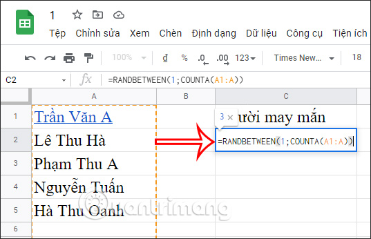
We have the association function =RANDBETWEEN(1;COUNTA(A1:A)), press Enter to get the result.

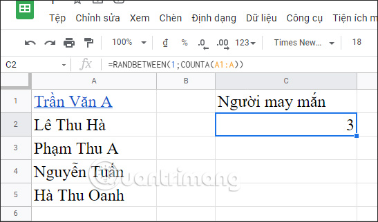
You will see the result 1 randomly selected number as shown below. This number can change randomly, corresponding to the name of the person on the list.

How to choose a random person in Google Sheets

In case you already have specific names of members and want to display the names of lucky people, you need to use the INDEX function.

The INDEX function will return the results of 1 specified cell with rows and columns, with the formula =INDEX(reference, row, column). In there:

• Reference: is the range of cells to be selected.
• Row (optional): is the row number in the range to return 1 cell reference.
• Column (optional): is the column number in the range to return 1 cell reference.

Applying to this problem, the Reference is a list of names to choose and choose a random number in the form of rows, from which to compare the name corresponding to the random number.

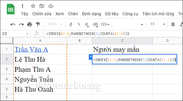
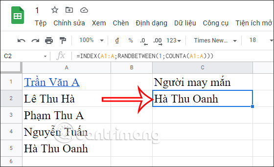
The recipe is =INDEX(A1:A;RANDBETWEEN(1;COUNTA(A1:A))). Specifically:

• A1:A is the range, the first argument to the INDEX function.
• Row here is the entire range RANDBETWEEN(1;COUNTA(A1:A), get specific values ​​from random results.

Apply to the Sheets table, enter the complete formula and press Enter.

The result will be 1 random person that you need to choose.

So with the combination of the RANDBETWEEN function with the COUNTA function and the INDEX function in Google Sheets, we can apply it to handle many different random number selection requirements.