How to use the Group feature in Excel

The Group feature in Excel is a feature that groups columns of data into one to easily perform operations such as hiding columns in Excel, similar to when we group shapes in Excel to freeze insertion shapes in Excel. When grouping columns of content, the actions will be applied to all columns or rows. In particular, we can use Excel keyboard shortcuts to work with merged columns. The following article will guide you to read how to group data columns in Excel.

Instructions for grouping columns and rows in Excel

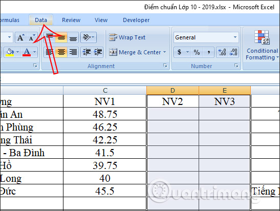
Step 1:

You then open the Excel table highlight the columns or rows you want to group into one. Then you click Data item on the toolbar in Excel.

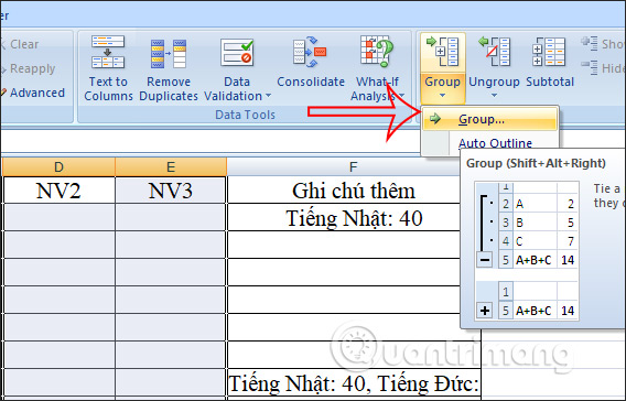
Step 2:

Then look down below to come Outline group then click on the Group option. Now showing the option to group columns, we click Group to make the group of 2 columns selected as 1.

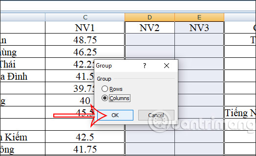
Then display the column group or row group selection table and click OK to execute.

Step 3:

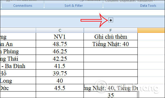
At this time, the top of the board will display a horizontal line with 2 dots in the grouped columns. To Quickly hide 2 columns this you just need to click minus sign icon is to be.

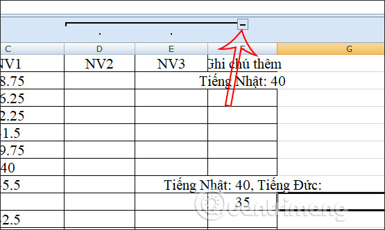
The 2-column results are hidden and if desired display again then the user just needs Click on the plus icon is to be.

Step 4:

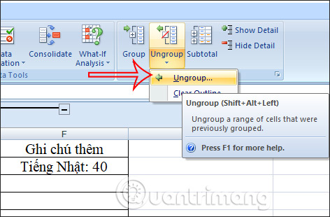
To cancel grouping of columns, first of all you need to Click on a column in the group then press Ungroup to cancel the group. Perform work with each remaining column in the group.

Excel keyboard shortcuts merge columns and rows in a table

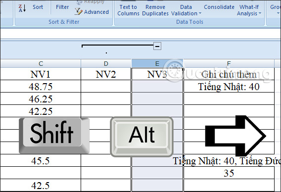
For faster execution we can use keyboard shortcuts. First of all you also Click on the column, first row want to group and press the key combination Shift + Alt + →. Continue Click on each remaining column and press the same key combination as above to group.

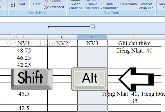
when the do not want to merge columns Again, click on the column and then click Shift + Alt + ← is done.