How to use the IMPORTRANGE function in Google Sheets

The IMPORTRANGE function in Google Sheets will help us link data from different spreadsheets, to search data quickly, get data according to the requirements displayed in the function. So you can use the IMPORTRANGE function to extract data, quickly link data in Google Sheets data tables. Using the IMPORTRANGE function in Google Sheets is also simple and can be combined with some functions in Google Sheets. The following article will guide you to use the IMPORTRANGE function in Google Sheets.

Instructions for using the Google Sheets IMPORTRANGE function

Function structure IMPORTRANGE Google Sheets =IMPORTRANGE(“spreadsheet_url”; “string_range”). Inside:

• Spreadsheet key: is a long string of numbers and letters in the URL for a given spreadsheet.
• Spreadsheet url: is the link address of a certain spreadsheet file.
• Range string: is the exact name of the worksheet that takes the data followed by ‘!’ and the range of cells you want to get data from.

We will take an example with the Grade 10-2019 Benchmark data table, with the request to extract data from cell B2 to cell C29 in the worksheet Page 1.

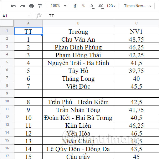
You open a completely new spreadsheet in Google Sheets to get the data of the spreadsheet you need. First you need to copy the link of the Class 10-2019 Grade Benchmark document.

Next at the new spreadsheet interface, we enter the function formula as below and then press Enter.

=IMPORTRANGE("https://docs.google.com/spreadsheets/d/19AGre5-Fvin6Z4D0bW6e4iq6yYX13kar0EIvXAVh-VQ/edit#gid=887314864"; "Page1!B2:C29")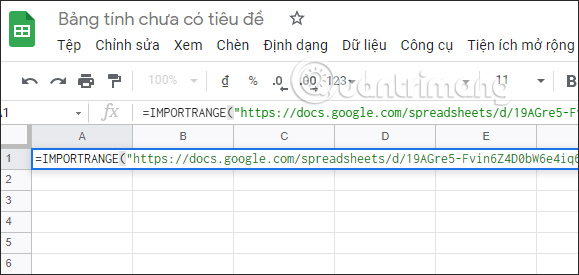

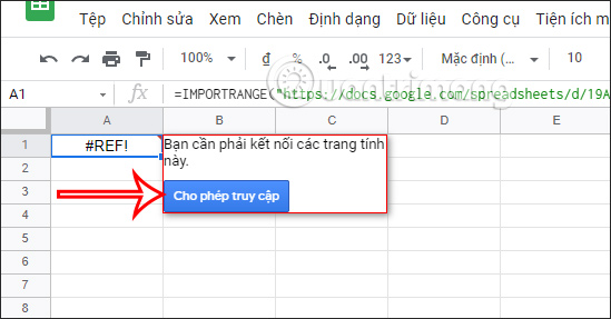
Immediately you will see newspaper #REF!. You need to click on this newspaper and press Allow access to allow the IMPORTRANGE function to access data from another sheet.

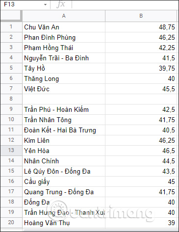
The data results from the sheet you selected are displayed in another sheet as shown below.

How to use the IMPORTRANGE function with the QUERY . function

When you combine the IMPORTRANGE function with the QUERY function, you can get the exact data according to the conditions to be extracted.

We will zone the data from cell B2 to cell C29 in the worksheet Page 1 and only take the NV1 column. You enter the formula as below and then press Enter.

=QUERY(IMPORTRANGE("https://docs.google.com/spreadsheets/d/19AGre5-Fvin6Z4D0bW6e4iq6yYX13kar0EIvXAVh-VQ/edit#gid=576960759";"Page1!B2:C29");"SELECT Col2")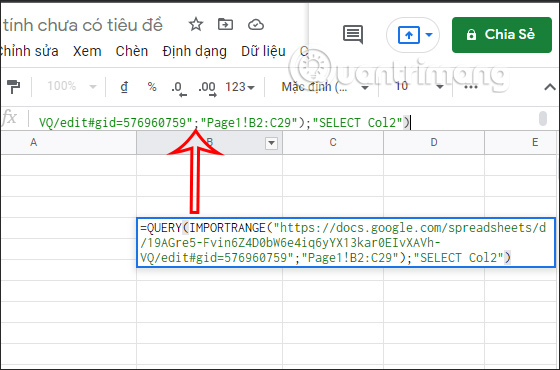 

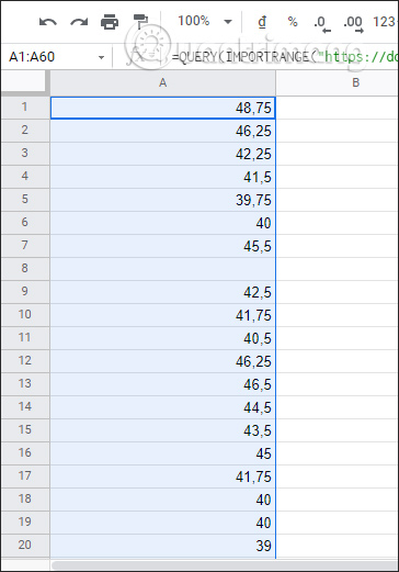
The results will only show the NV1 score column.

Or you can also take the score value of schools with scores NV1<40 for example.

We enter the function formula as below and then press Enter.

=QUERY(IMPORTRANGE("https://docs.google.com/spreadsheets/d/19AGre5-Fvin6Z4D0bW6e4iq6yYX13kar0EIvXAVh-VQ/edit#gid=576960759";"Page1!B2:C29");"Sect Col1 where Col2 <40")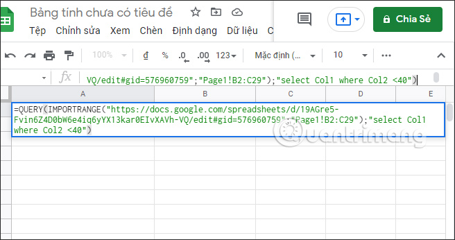 

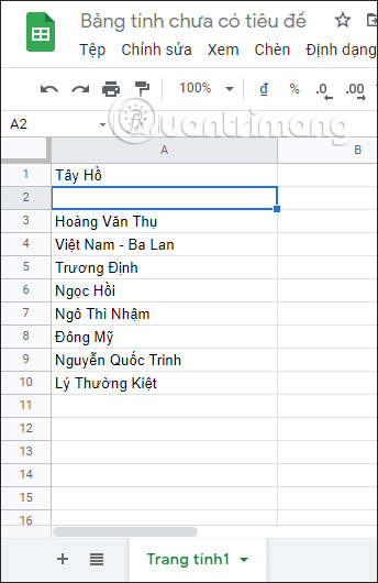
The results will show the names of schools with NV1 scores lower than 40 points.