How to use the UNIQUE function in Google Sheets

Usually, we import data into our spreadsheets from different sources. Whether online or from other software, there are bound to be instances where data is duplicated. In these cases, you will need to clean up your data to remove duplicate values, which can become very tedious to do manually.

In these cases, using the UNIQUE function in Google Sheets is a smart choice. This article will discuss the UNIQUE function, how to use it and combine it with other functions.

What is the UNIQUE function in Google Sheets?

The UNIQUE function in Google Sheets is a handy function that helps you find unique values ​​in a data set and remove any duplicates.

This function is ideal if you often work with large amounts of data. It allows you to find values ​​that appear only once in a spreadsheet. It works great with other important Google Sheets skills and functions. The UNIQUE function formula uses three arguments, but the cell range is the only required argument.

Syntax for UNIQUE function in Google Sheets

Here is the syntax to follow to use the UNIQUE function in Google Sheets:

=UNIQUE( range, filter-by-column, exactly-once)

This is what each argument represents:

• range – this is the address of the cell or range of data that you want to execute the function on.
• filter-by-column – this argument is optional and you use it to specify whether you want the data to be filtered by column or row.
• exactly-once – this is also an optional parameter and determines if you want non-duplicate entries. FALSE means you want to include unique values. TRUE means you want to remove entries with any number of duplicates.

To use formulas, make sure that you format the numeric values ​​correctly.

How to use the UNIQUE function in Google Sheets

Here are the steps you need to follow to use the UNIQUE function in Google Sheets:

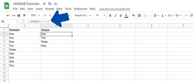
1. Click the blank cell where you want to enter the formula.

2. Enter =UNIQUE( to start the recipe.

3. Type or click and drag across the appropriate range of cells.

4. End the formula with a closing brace.

5. Press Enter to execute the formula.

Here is another example to demonstrate the UNIQUE formula.

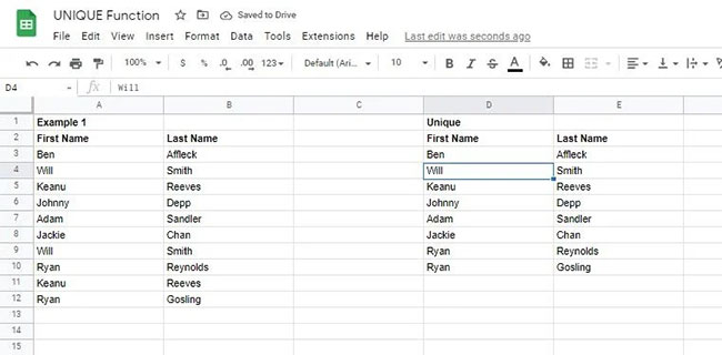
This example works with two columns instead of one. When executing the formula in the data, the formula will search for unique values ​​in two columns at the same time instead of searching each column.

You can observe this as Ryan Gosling and Ryan Reynolds. Although the two share the same name, they are unique, meaning the two values ​​are separate. Learning this function will also help you master the UNIQUE function in Excel.

Combine UNIQUE . function

Similar to most other functions in Google Sheets, the UNIQUE function can be paired with other formulas to enhance its functionality. Here are a few ways you can do this.

UNIQUE with SORT

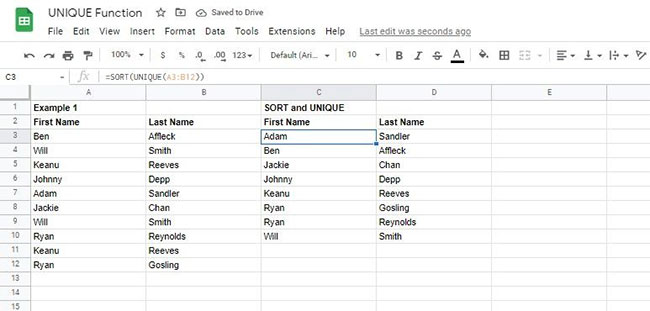
The article used one of the previous examples here. Using a UNIQUE formula with two columns provides the expected result. Now, use SORT with UNIQUE to find unique values ​​in the dataset and sort them alphabetically.

UNIQUE with TRANSPOSE

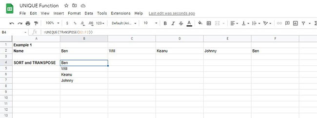
You can only use the UNIQUE function with vertical data, so you will need to convert the horizontal data to vertical before using the UNIQUE function on it. TRANSPOSE in Google Sheets works similar to Transpose in Excel. So you can use it to lay your output horizontally.

Make sure there is space required for the data to be displayed before writing the formula. If you want to convert the data back to its original form, use the TRANSPOSE function again.

Tips for UNIQUE . function

Here are some tips for using the UNIQUE function in Google Sheets:

• Make sure you provide enough space for the data set’s contents to be displayed. If the data cannot fit in the space provided, Google Sheets will display an error #REF!.
• If you want to clear all the values ​​that the UNIQUE function displays, delete the first cell where you enter the formula.
• If you want to copy the values ​​returned by the UNIQUE formula, copy them first with Ctrl + or by right clicking, clicking and selecting Copy. To paste the values:

1. Click Edit

2. Then enter Paste and Paste Special.

3. Click Paste values ​​only. The formula will be deleted and only the values ​​will be retained.

The UNIQUE function is a simple yet convenient function to use in Google Sheets, especially if you work with large spreadsheets.

You can use this function and many other Google Sheets features to calculate and make important business decisions.