Ranking using the RANK function in Excel is extremely simple with only 3 steps

Are you a teacher or someone who always needs to sort and classify data in Excel files? Then this is the post for you. Explore and learn about RANK function in Excel together GhienCongListen for your work to achieve results much faster.

What is the RANK function in Excel?

The RANK function in Excel is a function introduced for the purpose of sorting and classifying data and data. You can easily sort or rank your data from high to low or from low to high depending on your preference.

Advertisement

The RANK function is extremely popular with users when they need to work with a spreadsheet with lots of data or need to rank depending on the values ​​in the worksheet.

Syntax of RANK function in Excel

The RANK function in Excel has an extremely easy-to-remember formula:

Advertisement

• =RANK(value to sort, list or block of data to sort, [thứ tự cần xếp])

For the last argument [thứ tự cần xếp], you can omit this argument or enter zero, then Excel will default that you want to sort in order from highest to lowest. Conversely, if you want to sort in order from lowest to highest, the argument to fill will be 1.

How to use the RANK function in Excel and illustrative examples

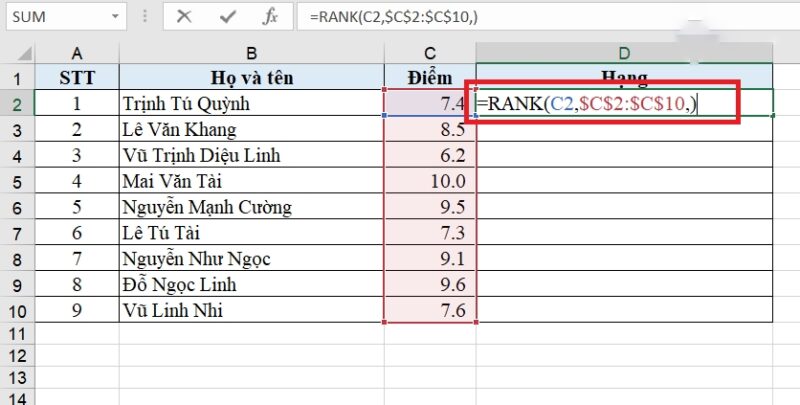
For example, you need to rank based on the average score for a list of students in the class like the example below:

Advertisement

At this point, the function formula you need to use will be:

In there:

• C2: the address of the cell containing the value to be ranked.
• $C$2:$C$10: List sequence containing values ​​in the same range to be ranked.
• Last argument left blank: by default Excel will rank by value from high to low.

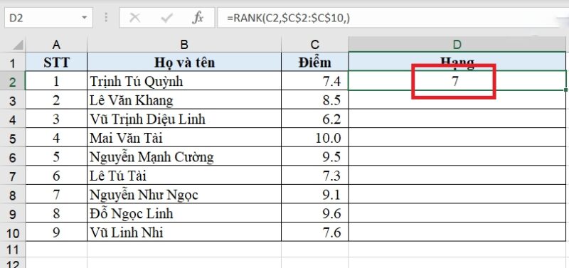
After pressing Enteryour function formula will return a value like the image below.

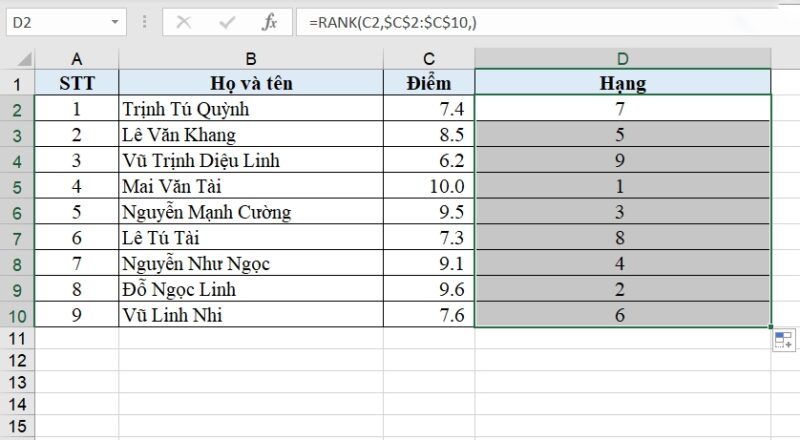
Copy the function formula to the remaining lines and you’re done:

Using the RANK function in Excel will make your ranking work much faster and more accurate.

Note when using the RANK function in Excel

Rank order control

With the ranking order, you can completely choose the number 0 or the number 1 to sort in order from high to low or from low to high. Depending on your sorting purpose, you can enter the appropriate arguments to get the result you want.

Duplicate

In case there are duplicate values, Excel will have the same rank and affect the ranking later. For example, if the number 9 appears twice, then both values ​​will have the same rank of 2 and now the number 8 will be the rank of 4 without the rank of 3.

Other Notes

When using the RANK function in Excel, you also need to be aware of the second argument, the list argument, or the data block to be sorted.

If in this argument you enter a range of values, you need to lock them with a keyboard shortcut F4 so that when copying the function formula to the next lines, these value addresses are not jumped, distorting the ranking of the values ​​in the sequence.

Not only teaching you how to use the RANK function in Excel, but GhienCongList also has many other posts to guide you about common functions that you can refer to:

After this post, the RANK function in Excel will help you a lot in any work related to numbers. Don’t forget to Like & Share the article and visit GhienCongListen more often!