How to change color of Excel cells according to conditions

Changing the color of Excel cells according to conditions is a simple way for us to easily identify or distinguish value cells in Excel tables. Previously, the Network Administrator has guided you to read many examples of cell coloring according to different conditions such as coloring blank cells in Excel, coloring alternating cells in Excel, changing alternating line colors in Excel… Users will use the Conditional Formatting cell formatting tool in Excel, and then enter the cell color change rule, depending on what you want to change the cell color for. The following article will give you a general guide on how to color Excel cells according to conditions.

Instructions to change the color of Excel cells according to conditions

Step 1:

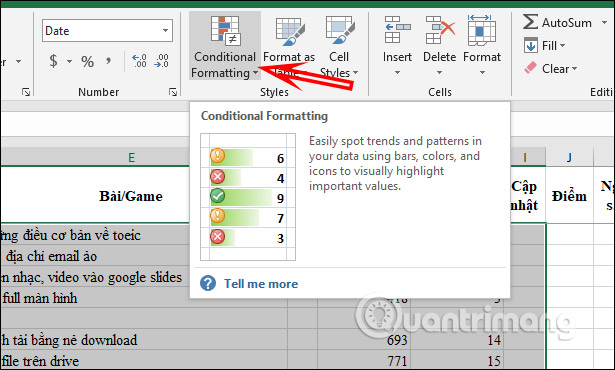
First of all, you need to highlight the data area you want to change color according to the condition, then click Conditional Formatting.

Step 2:

You will now see 2 options: available conditional formatting and custom conditional formatting.

As long as it’s available, you’ll have the option to:

• Highlight Cells Rules: Highlight cells by value.
• Top/ Bottom, Rules: Identify cells by rating.
• Data Bars: Display cells according to the size of the value.
• Color Scales: Color large and small values.
• Icon Sets: Add icons to cells by value.

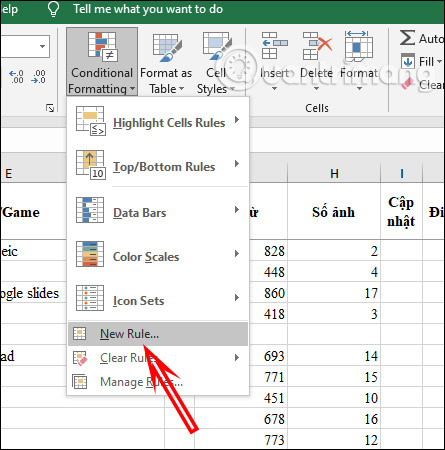
With own conditional formatting options then the user can choose to color the cell according to the conditions they enter themselves. Click New Rule… to add a new condition.

Step 3:

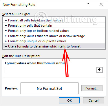
Later in the Select a Rule Type you click on the item Use a formula to determine which cells to format. Afterward enter the cell format formula at Format values ​​where this formula is true. For example, to color alternate lines, enter the formula =MOD(ROW()/2,1)>0.

Keep pressing Format button to select the color for the entered condition.

Step 4:

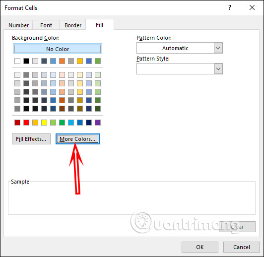
Now you click Item Fill already Select the color you want to change for the cell. If you want to add another color, click More Colors below. Finally click OK to change the color.

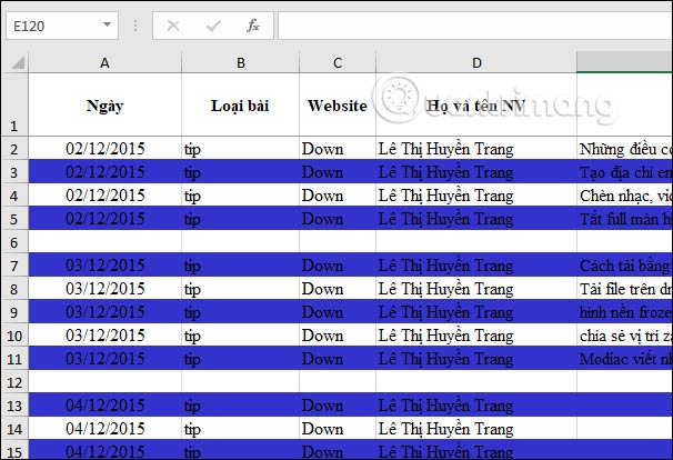
The resulting data table is colored as shown below.

Step 5:

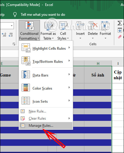
In case you want change cell colorpress Conditional Formatting then choose Manage Rules…

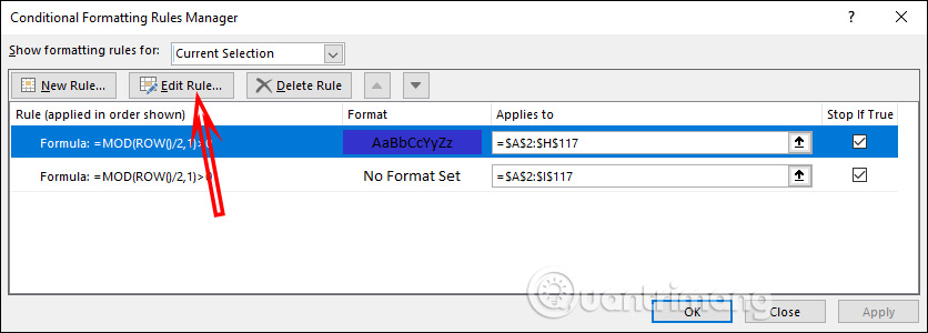
Click Conditions for wanting to change the color already Click Edit Rule… At this point you also need to click Format then change to another color you want.