Lesson 32: How to use Split (split) worksheets in Excel

Split (split) your worksheet to view multiple parts of the worksheet at once in Excel. You can split the sheet into 2 parts, the upper part and the lower part by the following way.

How to use Split in Excel

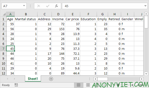
1. First, select a cell in column A.

2. On the View tab, in the Windows group, select Split.

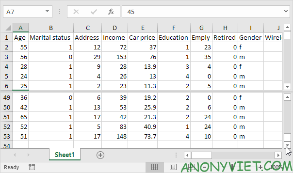
3. Notice the two vertical scroll bars. For example, use the bottom vertical scroll bar to move to row 49. As you can see, the first 6 rows are still visible.

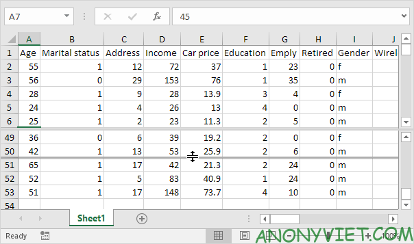
4. To change the layout, use the horizontal divider to adjust it to your liking.

5. To remove split, simply double click on the horizontal split bar.

Note: in a similar way, you can split your window into left and right areas by selecting a cell in row 1 before clicking View -> Split. You can even split your window into 4 regions by selecting a cell that is not column A or row 1. Any changes you make to one area are immediately reflected in the other zones. .

In addition, you can also see many other excel articles here.