Cover 44: How to Customize Number Formats in Excel

Excel has many preset formats that you can use such as Currency, Accounting, Date, Time, Percentage, .. If you cannot find the right format, you can customize the format as shown in the article below. This.

How to Customize Number Formats in Excel

Automatically add leading zeros

For example: you want to enter 5 digits. Instead of entering 00041, simply enter 41 and Excel will automatically add leading zeros.

first. Enter the value 41 in cell A1.

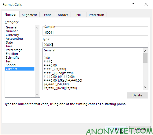
2. Select cell A1, right-click and select Format Cells.

3. Select Custom.

4. Enter the following number format code: 00000

5. Click OK.

Note: Excel gives you a preview of the format in Sample.

Result:

Note: cell A1 still contains the number 41. We only change the display of this number, not the value of cell A1.

Decimal place

You can also control the number of decimal places. Use 0 to display the nearest integer value. Use 0.0 for one decimal place. Use 0.00 for two decimal places,..

first. Enter the value 839.1274 in cell A1.

2. Use the following number format code: 0.00

Insert text

You can also add text to your number. For example, add “ft”.

first. Enter the value 839.1274 in cell A1.

2. Use the following number format code: 0.0 “ft”

Note: I only changed the display of this number, not its value. You can still use this number for calculations.

Big number

You can also control large numbers. Use one comma (,) to display thousands and use two commas (,,) to display millions.

first. Enter the following values ​​in cells A1, B1, C1 and D1: 1000000, 2500000, 81000000, and 700000.

2. Use the following number format code: 0.0 ,, “M”

Note: we used 0.0 for one decimal place and “M” to add the letter M.

Repeat character

Use asterisks

include a character to tell Excel how many times you want the character to be repeated. first.

Enter Hi in cell A1. 2. Use the following number format code:

Cover 44: How to Customize Number Format in Excel 20

Note: the @ symbol is used to enter text.

Color

You can control positive numbers, negative numbers, zeros and text at the same time! Each part is separated by a semicolon (;) in the number format code. first.

Enter the following values ​​in cells A1, B1, C1 and A2: 5000000, 0, Hi, and -5.89. 2. [Green] Use the following number format code: [Red] $ #, ## 0 _); [Blue] $ (#, ## 0); “zero”;

Cover 44: How to Customize Number Format in Excel 21 Note:

#, ## are used to add commas to large numbers. To add a space, use an underscore “_” followed by a character. The length of the space will be the length of this character. In my example, I added a single quote “)”.

Date and time

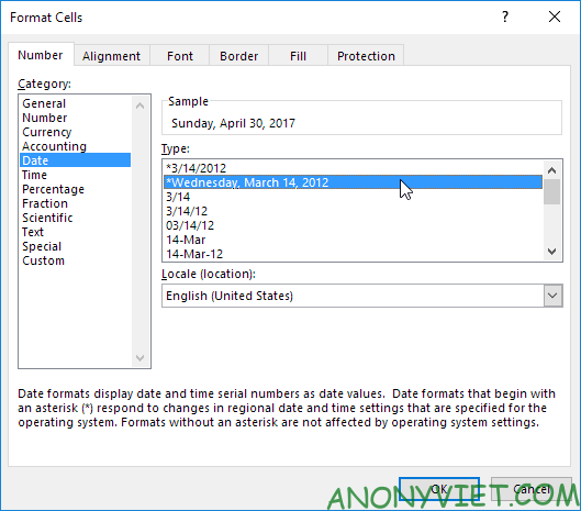
You can also control the date and time. Use one of the existing Date and Time formats to get started. first.

Enter the value 42855 in cell A1. 2.

Select cell A1, right-click, and then select Format Cells. 3.

Cover 44: How to Customize Number Format in Excel 22

Note: Excel gives you a preview of the date in Sample. 4.

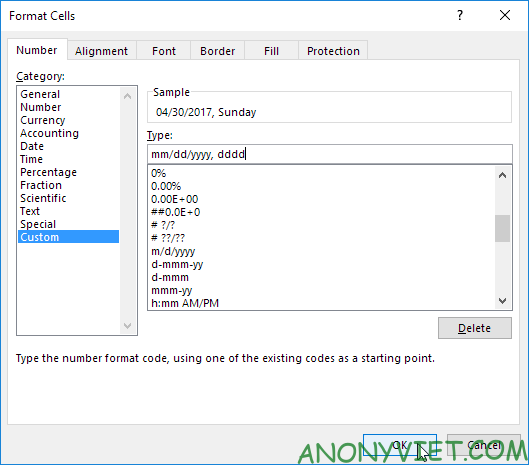
Select Custom. 5.

Slightly change the format code to: mm / dd / yyyy, dddd 6.

Cover 44: How to Customize Number Format in Excel 23

Cover 44: How to Customize Number Format in Excel 24

In addition, you can also see many other excel articles here.