How to create a pie chart in Google Sheets

Graphs and charts give you visual ways to represent data. So if you want to show parts of the overall data, a pie chart is the way to go. You can create and customize pie charts in Google Sheets easily.

How to create a pie chart in Google Sheets

Creating charts in Google Sheets is much simpler than you think. Select the data you want to use for the chart. Then click Insert > Chart.

You will immediately see a suggested chart appear based on your data. It might be a pie chart, but if not, you can change it easily.

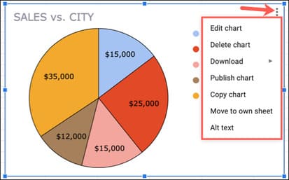
Select the chart and click on the three dots shown at the top right. Click “Edit Chart” to open the Chart Editor menu.

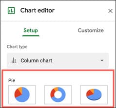
On the Setup tab, click Chart Type. Scroll down to the Pie section and select the pie chart style you want to use. You can choose a pie chart, a Donut chart, or a 3D pie chart.

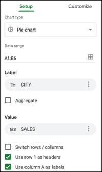
You can then use other options on the Setup tab to adjust the data range, convert rows and columns, or use the first row as the header.

Customize pie charts in Google Sheets

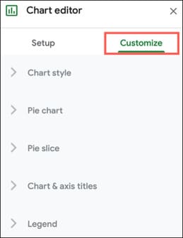
Click the Customize tab in the Chart Editor menu. You will see several sections; Most are available for all chart types you use in Google Sheets.

In Chart Styleyou can choose background color, font style, and chart border color.

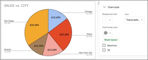
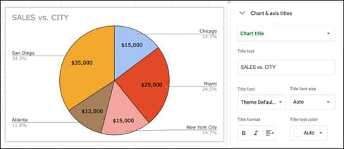
In section Chart & Axis Titlescan change the title, add subtitles and font format.

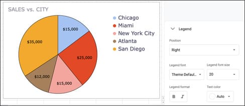
In Legendyou can position the legend and choose the font style, size, format, and color.

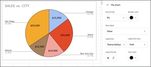
For pie charts in particular, you have two additional pieces to work with: Pie Chart and Pie Slice. These areas allow you to customize as you wish.

In Pie Chart, add and adjust the center, or choose a border color for the chart. You can then add labels to individual slices if desired. You can customize from Label, Value, Percent or Value. If you add slice labels, you can customize the font style, size, format, and color.

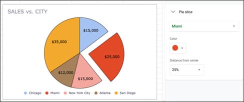
In section Pie Slice, you can change the color of each slice by choosing from the drop-down list, then choosing a color below. You can also use Distance From Center to make specific slices separate from the center of the graph.

Additional charting options

You can move the chart by selecting and dragging it to where you want it. You can also resize the chart by dragging the corner.

If you want to delete the chart, download, publish, copy or move it, or add alt text, click the three dots at the top right of the chart.

Google Sheets makes it easier to create and customize charts. Alternatively, you can also rename columns or rows in Google Sheets here.