Lesson 70: How to create a drop-down menu in Excel

Drop-down menus (also known as drop-down lists) in Excel are useful if you want to make sure that users are only allowed to select one item from the list, instead of entering their own value.

1. On the second sheet, enter the items you want to appear in the drop-down list.

Note: if you don’t want users to access the items on Sheet2, you can hide Sheet2. By right clicking on Sheet2 and clicking Hide.

2. On the first sheet, select cell B1.

3. On the Data tab, in the Data Tools group, click Data Validation.

4. In Allow, click Custom.

5. In Formula, enter the formula shown below and click OK.

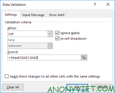
6. Click OK.

Result:

Note: to copy/paste the dropdown, select the cell with the dropdown and press CTRL+c, select another cell and press CTRL+v.

7. You can also import content directly into Source.

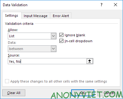
Note: Your drop-down list is case sensitive. For example, if the user enters yes, an error warning will be displayed.

Allow other content input

You can also create a drop-down list in Excel to allow users to enter other content.

1. First, if you enter a value that is not in the list, Excel will display an error warning.

2. On the Data tab, in the Data Tools group, click Data Validation.

3. On the Error Alert tab, uncheck ‘Show error alert after invalid data is entered’.

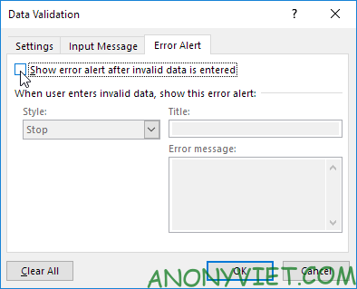
4. Click OK.

5. You can now enter a value that is not in the list.

Add/Remove items in the list

You can add or remove items from the drop-down list in Excel without opening the ‘Data Validation’ dialog box and changing the reference. This will help save time.

1. To add an item to the drop-down list, go to sheet2 and select an item.

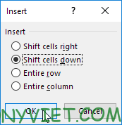
2. Right-click, and then click Insert.

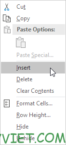
3. Select “Shift cells down” and click OK.

Result:

Note: Excel automatically changed the reference from Sheet2!$A$1:$A$3 to Sheet2!$A$1:$A$4. You can check this by opening the ‘Data Validation’ dialog box.

4. Enter a new entry.

Result:

5. To remove an item from the drop-down list, in step 2, click Delete, select “Shift cells up” and click OK.

Dynamic list

You can also use a formula that automatically updates the drop-down list when you add an item to the end of the list.

1. On the first sheet, select cell B1.

2. On the Data tab, in the Data Tools group, click Data Validation.

3. In Allow, click Custom.

4. Click Source and enter the formula: =OFFSET (Sheet2!$A$1,0,0,COUNTA(Sheet2!$A:$A,1)

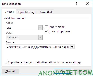
5. Click OK.

6. On the second page, simply add a new item to the bottom of the list.

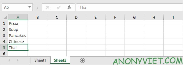
Result:

Remove drop-down list

1. Select the cell with the drop-down list.

2. On the Data tab, in the Data Tools group, click Data Validation.

3. Click Clear All.

Note: to remove all other drop-down lists with the same settings, select “Apply these changes to all other cells with the same settings” before you click Clear All.

4. Click OK.

List of dependencies

1. For example, if the user selects Pizza from the first drop-down list.

2. The second drop-down list will contain Pizza items.

3. But if the user selects Chinese from the first dropdown, the second dropdown will contain Chinese dishes.

You can read this article to know how to create a dependency list. In addition, you can also see many other excel articles here.