[Tuts] Instructions on how to use the VLOOKUP function in Excel

In the Excel application, functions are used to support the calculation and sorting of lists and values.. helping us to achieve absolute accuracy in calculations. And as you all know, in recent articles, I have introduced to you a number of functions, such as the LEN function, the MID function, the YEAR function, the TODAY function or the RANK function.

To help you have more choices and be able to meet the needs of creating diverse statistics, in this article, I will show you how to use the VLOOKUP function, a function that detects find the absolute, and relative argument values ​​contained in the list.

Okay, so that you don’t have to wait too long, let’s start this practice right now 😀

Read more:

I. Formula using VLOOKUP . function

The VLOOKUP function formula is as follows: VLOOKUP(lookup_value,table_array,col_index_num,[range_lookup])

In there:

• lookup_value: Value to bring to the search.
• table_array: Table of probe values, this table we leave in the form of Absolute address (by highlighting the probe table and pressing the F4 key)
• col_index_num: Column to detect.
• range_lookup: As the search range, TRUE is equivalent to the value 1 (relative detection), FALSE is equivalent to the value 0 (absolute detection, and usually we will use this absolute value).

AND here I will rewrite the formula in a way that is easier to understand (in my opinion )

• VLOOKUP(Value to take away, probe table, probe column, 0)

II. Example of using the VLOOKUP function in Excel

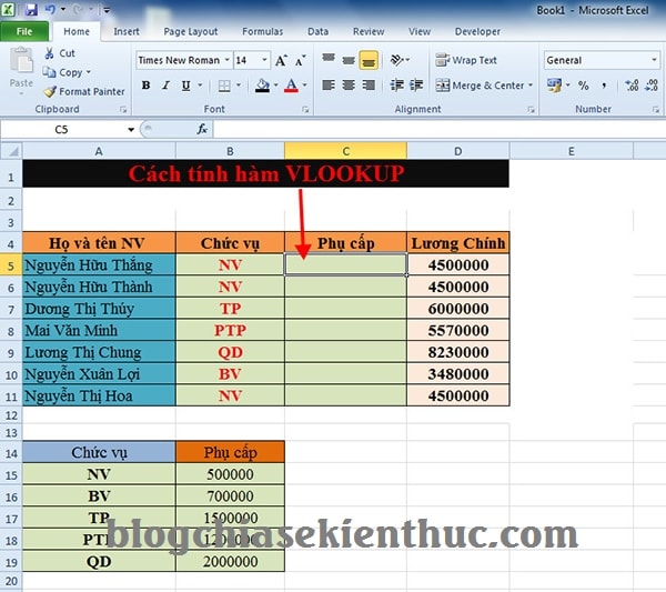
+ Step 1: You turn on your Excel application. For example, I will have an Excel table as shown below.

Including the value you want to find, and the argument value you want to find. Corresponding as shown below, then you select the first cell to enter the formula.

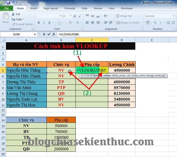
+ Step 2: In the first cell of the value to find you enter the formula =VLOOKUP( then click on the search value in the column, search (here the column position).

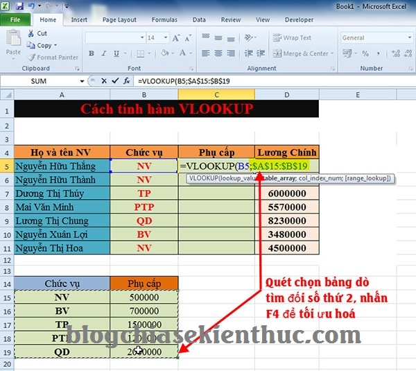
+ Step 3: Enter a comma ( , ) or semicolon ( ; )depending on the Excel version to break the argument and scan the entire corresponding detection value below.

Then press the key F4 to absolute table lookup.

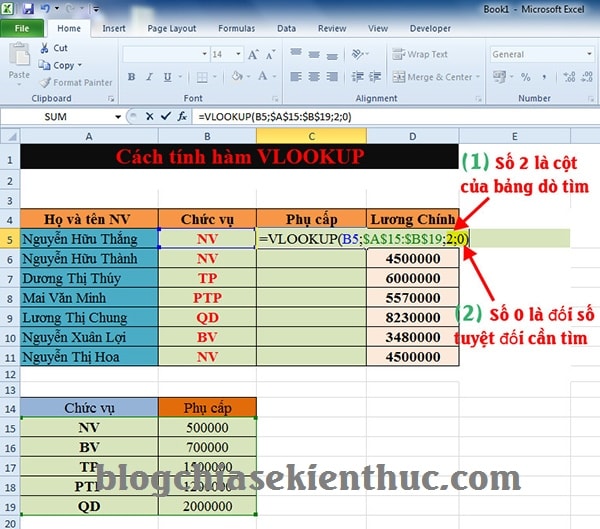
+ Step 4: Then you continue to use commas ( , ) or semicolon ( ; ) to pass arguments.

And you enter the number 2, corresponding to the number of columns is 2 from left to right.

In case there are many columns and values ​​to find, you can change the number to 3 or greater than 3. In general, you just need to count from left to right to count the number of columns.

Then enter a semicolon ( , ) and enter the number 0 (absolute value) or 1 (relative value). Finally you close the parenthesis and press Enter to produce results.

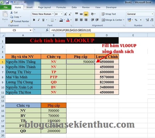
Finally we get the complete formula as follows: =VLOOKUP(B5;$A$15:$B$19;2;0)

+ Step 5: Once you have found the value you are looking for with the VLOOKUP function for a cell, it’s now simple.

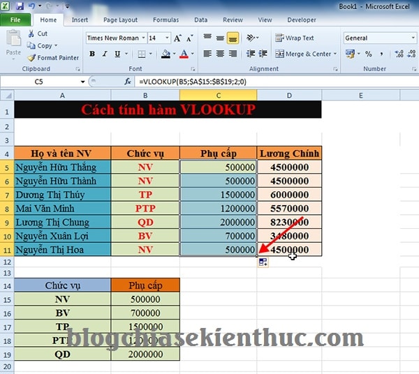
You proceed to Copy the formula for the remaining cells and you’re done, click on the cell with the formula you just entered => move the mouse to the bottom right corner of that cell until a small plus sign of the cell that has calculated the formula appears => Fill the entire list as shown.

And we have the same result.

Epilogue

OK, here I just finished the tutorial for you How to use the VLOOKUP function in Excel to detect the value and return the corresponding value in the spreadsheet quickly and easily.

Really, this VLOOKUP function is extremely useful for accountants, your use of this VLOOKUP function will save you a lot of time in your work as well as in the learning and calculation process.

Hopefully with the knowledge that I share today will be useful and useful to you. Good luck !

CTV: Luong Trung – techtipsnreview