
In the process of data statistics, it is not uncommon for us to encounter “infinitely long” spreadsheets. This makes it very difficult for you to capture and manage the information contained in that Excel file.
Therefore, to assist you in managing Excel files more effectively, in this article, I will share with you how to shorten the spreadsheet with the SCROLL BAR bar.
Job Collapse Excel spreadsheet within a certain range will make it more convenient for you to aggregate and manage your Excel files.
Read more:
How to collapse a spreadsheet using the SCROLL BAR . scrollbar
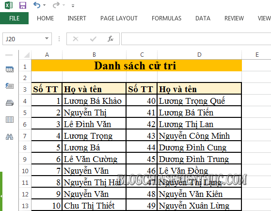
+ Step 1: First, you click to open the Excel file that needs to be processed.
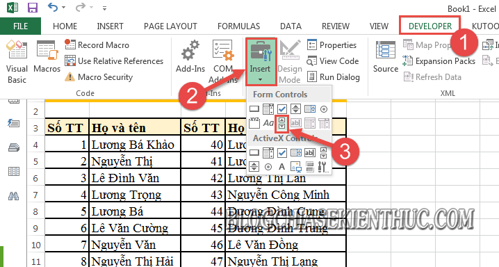
+ Step 2: Here, you click to open the Developer tab => and select Insert => choose next Scroll Bar (From Control).
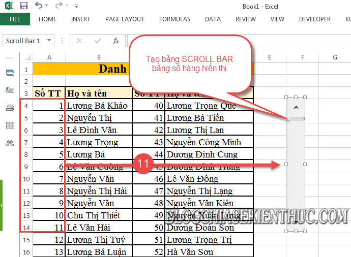
+ Step 3: Then you make a line SCROLL BAR corresponding to the number of rows shown on the worksheet that you want by holding down the left mouse button and dragging down.
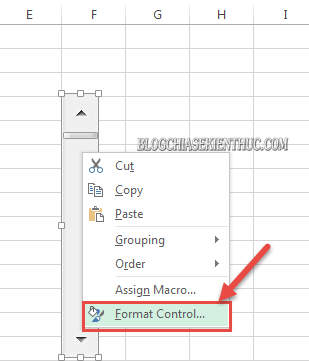
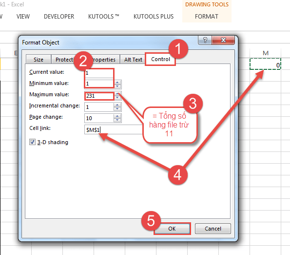
+ Step 4: Then you right click on the bar SCROLL BAR => and choose Format Control....
+ Step 5: At the dialog box Format Controlyou click open tab Control => then set the value as follows:
- Current value =
1. - Minimum value =
1. - Maximum value = (the total number of rows on the worksheet minus the number of rows shown in the SCROLL BAR bar).
- Cell Link: You click on any cell on the spreadsheet to establish a connection.
=> Then you press OK to apply.
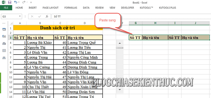
+ Step 6: Next, highlight the worksheet title area => and right-click and select Copy.
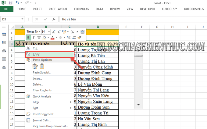
Then Paste to the side of the SCROLL BAR bar as shown.
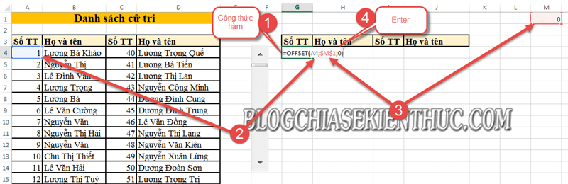
+ Step 7: Okay, now you enter the function formula =OFFSET in the box below the title box as follows => then press Enter to execute.
=OFFSET(show cell value;cell containing the spreadsheet link;0)
In there:
- Cell containing the spreadsheet link: After selecting the cell containing the spreadsheet link, press the . key F4 on the keyboard to fix it.
- 0 is the absolute value !
Specific examples: =OFFSET(A4;$M$1;0)
+ Step 8: Then you keep the small plus sign in the formula cell => then Fill the formula down horizontally, and vertically as shown to apply the formula to the remaining cells.
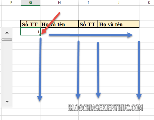
Finally we get the result as shown below. Here you can black out the display area and change the Fonts, font color, as well as the font size that will be displayed in the miniature spreadsheet….

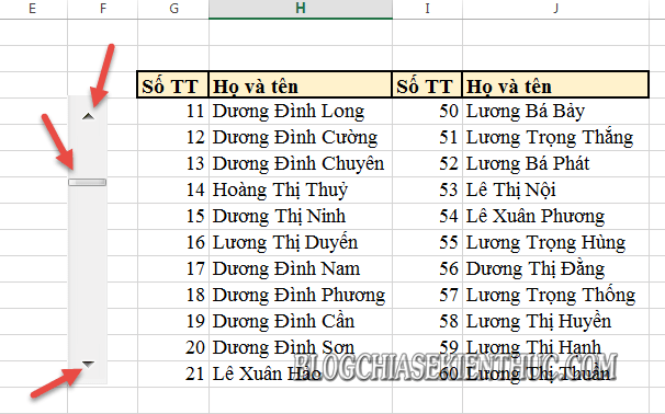
+ Step 9: And now you can use the mouse to drag the slider at SCROLL BAR, or click the triangle button above, or below to move the values up, down… to quickly review the information on the spreadsheet. .
Epilogue
Okay, that’s it, I just gave you a very detailed guide how to collapse an Excel spreadsheet with the SCROLL BAR . tool to make it easier to summarize and review information on Excel spreadsheets.
At this point, the tutorial on how to shorten the Excel spreadsheet with my SCROLL BAR bar will also be paused. Hope this little tip is helpful to you.
Good luck !
CTV: Luong Trung – techtipsnreview
Note: Was this article helpful to you? Don’t forget to rate the article, like and share it with your friends and family!
Source: How to collapse an Excel spreadsheet with the SCROLL BAR . scrollbar
– TechtipsnReview