Lesson 225: Data Bars in Excel

This article will show you how to use data bars in Excel.

Data bar

This article will guide you to create data bars in excel

1. Select range

2. On the Data panel in the Styles section, select Conditional Formating

3. Select Databars -> subtype

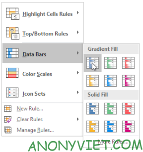
Result:

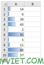
4. Change value

Result:

5. Select range A1:A10

6. On the Data panel in the Styles section, select Conditional Formating

7. Select edit rules

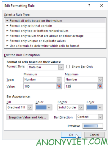
It will appear a table and you can edit your data bar there

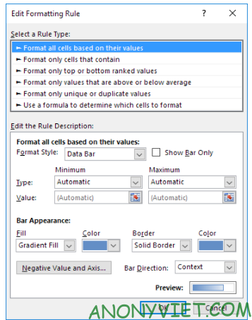
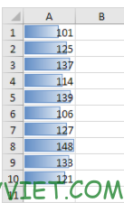
8. Select Number in the Minimum down-arrow list box and enter the value 100 and select Number in the Maximum drop-down arrow box and enter 150

9. Multiply OK 2 times

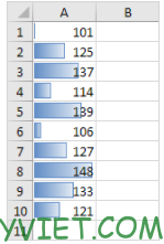
Result:

In addition, you can also see many other excel articles here.